Chapter 23 Best Subset Model Selection with Training/Test Set
As mentioned, it is not always best to include every variable into the linear regression model. We need to select the best subset of variables to include. The best subset algorithm exhausts every possible combination to select the best model of each size. However, this algorithm cannot be scaled up, so we use forward selection, which will add variables sequentially.
The forward model selection will generate \(p\) different models with distinct model size from \(1, 2, ..., p\), where \(p\) is the total number of independent variables. Thus, we need to choose the best model among these \(p\) models.
Previously, we used adj-R2, Cp, AIC and BIC for model selection. In this chapter, we will use training and test set to select the best model.
23.1 Create training/test set
There is no definitive rule on how much proportation of data goes to training set or test set. A typical rule of thumb is 80% of data goes to training set and 20% goes to test set.
Boston=fread("data/Boston.csv")             # load the data into R
Boston[,location:=factor(location)]
Boston[,chas:=factor(chas)]

num_row=nrow(Boston)  # check the number of rows

# Random select the training set
set.seed(1) # set the rand seed to ensure replicability

train_size=round(0.8*num_row,0)  # set the size of training set

# randomly select train_size=300 numbers from the sequence of 1 to nrow(Boston)=506
train=sample(1:num_row, train_size, replace=FALSE)

# the training set: Boston[train]
head(Boston[train])
## crim zn indus chas nox rm age dis rad tax ptratio black lstat
## 1: 0.10959 0 11.93 0 0.573 6.794 89.3 2.3889 1 273 21.0 393.45 6.48
## 2: 0.28392 0 7.38 0 0.493 5.708 74.3 4.7211 5 287 19.6 391.13 11.74
## 3: 2.01019 0 19.58 0 0.605 7.929 96.2 2.0459 5 403 14.7 369.30 3.70
## 4: 0.32543 0 21.89 0 0.624 6.431 98.8 1.8125 4 437 21.2 396.90 15.39
## 5: 25.94060 0 18.10 0 0.679 5.304 89.1 1.6475 5 666 20.2 127.36 26.64
## 6: 4.34879 0 18.10 0 0.580 6.167 84.0 3.0334 5 666 20.2 396.90 16.29
## location medv
## 1: south 22.0
## 2: west 18.5
## 3: north 50.0
## 4: east 18.0
## 5: west 10.4
## 6: south 19.9## crim zn indus chas nox rm age dis rad tax ptratio black
## 1: 0.02985 0.0 2.18 0 0.458 6.430 58.7 6.0622 3 222 18.7 394.12
## 2: 0.08829 12.5 7.87 0 0.524 6.012 66.6 5.5605 5 311 15.2 395.60
## 3: 0.21124 12.5 7.87 0 0.524 5.631 100.0 6.0821 5 311 15.2 386.63
## 4: 0.17004 12.5 7.87 0 0.524 6.004 85.9 6.5921 5 311 15.2 386.71
## 5: 0.22489 12.5 7.87 0 0.524 6.377 94.3 6.3467 5 311 15.2 392.52
## 6: 0.11747 12.5 7.87 0 0.524 6.009 82.9 6.2267 5 311 15.2 396.90
## lstat location medv
## 1: 5.21 south 28.7
## 2: 12.43 west 22.9
## 3: 29.93 north 16.5
## 4: 17.10 north 18.9
## 5: 20.45 north 15.0
## 6: 13.27 north 18.923.2 Evaluate the Best subset regression through training/test set
# find best subset based on training data
fwd_fit=regsubsets(medv~., data=Boston[train,], nvmax=18, method="forward")
fwd_fit_sum=summary(fwd_fit)
fwd_fit_sum
## Subset selection object
## Call: regsubsets.formula(medv ~ ., data = Boston[train, ], nvmax = 18,
## method = "forward")
## 16 Variables (and intercept)
## Forced in Forced out
## crim FALSE FALSE
## zn FALSE FALSE
## indus FALSE FALSE
## chas1 FALSE FALSE
## nox FALSE FALSE
## rm FALSE FALSE
## age FALSE FALSE
## dis FALSE FALSE
## rad FALSE FALSE
## tax FALSE FALSE
## ptratio FALSE FALSE
## black FALSE FALSE
## lstat FALSE FALSE
## locationnorth FALSE FALSE
## locationsouth FALSE FALSE
## locationwest FALSE FALSE
## 1 subsets of each size up to 16
## Selection Algorithm: forward
## crim zn indus chas1 nox rm age dis rad tax ptratio black lstat
## 1 ( 1 ) " " " " " " " " " " " " " " " " " " " " " " " " "*"
## 2 ( 1 ) " " " " " " " " " " "*" " " " " " " " " " " " " "*"
## 3 ( 1 ) " " " " " " " " " " "*" " " " " " " " " "*" " " "*"
## 4 ( 1 ) " " " " " " " " " " "*" " " "*" " " " " "*" " " "*"
## 5 ( 1 ) " " " " " " " " " " "*" " " "*" " " " " "*" "*" "*"
## 6 ( 1 ) " " " " " " " " "*" "*" " " "*" " " " " "*" "*" "*"
## 7 ( 1 ) " " " " " " "*" "*" "*" " " "*" " " " " "*" "*" "*"
## 8 ( 1 ) " " "*" " " "*" "*" "*" " " "*" " " " " "*" "*" "*"
## 9 ( 1 ) " " "*" " " "*" "*" "*" " " "*" " " " " "*" "*" "*"
## 10 ( 1 ) " " "*" " " "*" "*" "*" " " "*" "*" " " "*" "*" "*"
## 11 ( 1 ) "*" "*" " " "*" "*" "*" " " "*" "*" " " "*" "*" "*"
## 12 ( 1 ) "*" "*" " " "*" "*" "*" " " "*" "*" " " "*" "*" "*"
## 13 ( 1 ) "*" "*" " " "*" "*" "*" " " "*" "*" " " "*" "*" "*"
## 14 ( 1 ) "*" "*" "*" "*" "*" "*" " " "*" "*" " " "*" "*" "*"
## 15 ( 1 ) "*" "*" "*" "*" "*" "*" "*" "*" "*" " " "*" "*" "*"
## 16 ( 1 ) "*" "*" "*" "*" "*" "*" "*" "*" "*" "*" "*" "*" "*"
## locationnorth locationsouth locationwest
## 1 ( 1 ) " " " " " "
## 2 ( 1 ) " " " " " "
## 3 ( 1 ) " " " " " "
## 4 ( 1 ) " " " " " "
## 5 ( 1 ) " " " " " "
## 6 ( 1 ) " " " " " "
## 7 ( 1 ) " " " " " "
## 8 ( 1 ) " " " " " "
## 9 ( 1 ) "*" " " " "
## 10 ( 1 ) "*" " " " "
## 11 ( 1 ) "*" " " " "
## 12 ( 1 ) "*" " " "*"
## 13 ( 1 ) "*" "*" "*"
## 14 ( 1 ) "*" "*" "*"
## 15 ( 1 ) "*" "*" "*"
## 16 ( 1 ) "*" "*" "*"Again, summary(fwd_fit) narrows down to 16 different models with distinct model size. Now let’s examine which model results in the best out-of-sample predication over the test set.
Construct test set in the same format of training set:
##   (Intercept)    crim   zn indus chas1   nox    rm   age    dis rad tax ptratio
## 1           1 0.02985  0.0  2.18     0 0.458 6.430  58.7 6.0622   3 222    18.7
## 2           1 0.08829 12.5  7.87     0 0.524 6.012  66.6 5.5605   5 311    15.2
## 3           1 0.21124 12.5  7.87     0 0.524 5.631 100.0 6.0821   5 311    15.2
## 4           1 0.17004 12.5  7.87     0 0.524 6.004  85.9 6.5921   5 311    15.2
## 5           1 0.22489 12.5  7.87     0 0.524 6.377  94.3 6.3467   5 311    15.2
## 6           1 0.11747 12.5  7.87     0 0.524 6.009  82.9 6.2267   5 311    15.2
##    black lstat locationnorth locationsouth locationwest
## 1 394.12  5.21             0             1            0
## 2 395.60 12.43             0             0            1
## 3 386.63 29.93             1             0            0
## 4 386.71 17.10             1             0            0
## 5 392.52 20.45             1             0            0
## 6 396.90 13.27             1             0            0
Note: model.matrix() is a function to create a matrix which has the same columns as the regression dataset based on a formula.
Compute the out-of-sample prediction error based on test set:
#Initialize the vector for saving the mse (mean square error) err over the test set:
test_set_mse=rep(NA,16)

for(i in 1:16){

  coefi=coef(fwd_fit,id=i)

  # compute the out-of-sample prediction for model i
  pred=test_set[,names(coefi)]%*%coefi

  # compute the MSE for model i
  test_set_mse[i]=mean((Boston$medv[-train]-pred)^2)

}
Calculate rMSE and choose the best model to minimize rMSE:
test_set_rmse=sqrt(test_set_mse)
plot(test_set_rmse,ylab="Root MSE", type="b")
opt_id=which.min(test_set_rmse)
points(opt_id,test_set_rmse[opt_id],pch=20,col="red")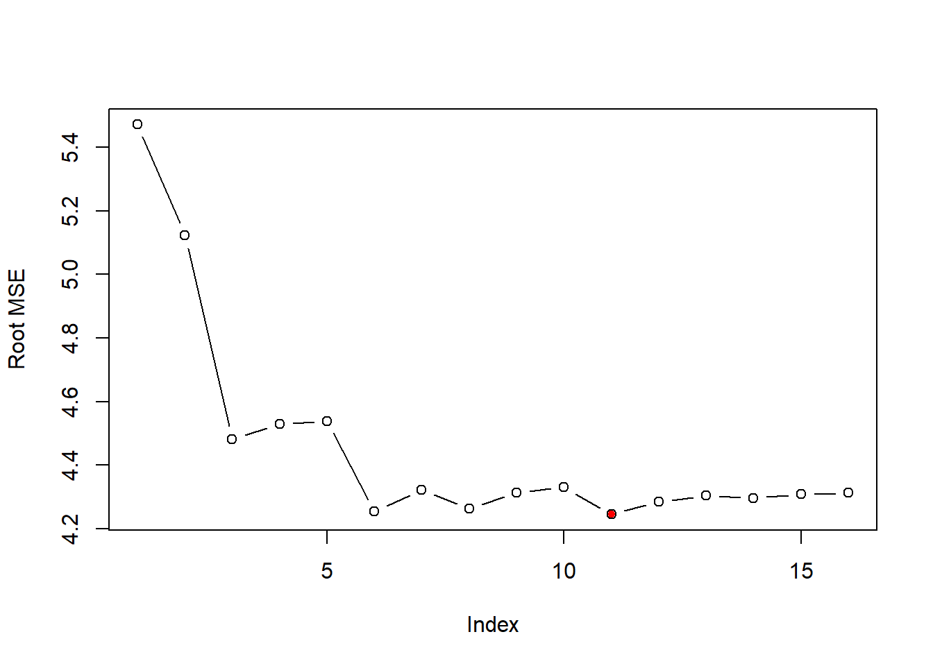 Observation: which model to choose? – the model with 11 variables, it minimizes the out-of-sample prediction.
##   (Intercept)          crim            zn         chas1           nox
##  22.322359524  -0.042315405   0.037742595   3.464838748 -14.551045654
##            rm           dis           rad       ptratio         black
##   4.472611255  -1.343541190   0.464600981  -0.748560817   0.009929678
##         lstat locationnorth
##  -0.559735879   1.123935544
Plot the optimal out-of-sample prediction:
coefi=coef(fwd_fit,id=opt_id)
opt_pred=test_set[,names(coefi)]%*%coefi

plot(Boston$lstat[-train], Boston$medv[-train])
points(Boston$lstat[-train], opt_pred,col="blue")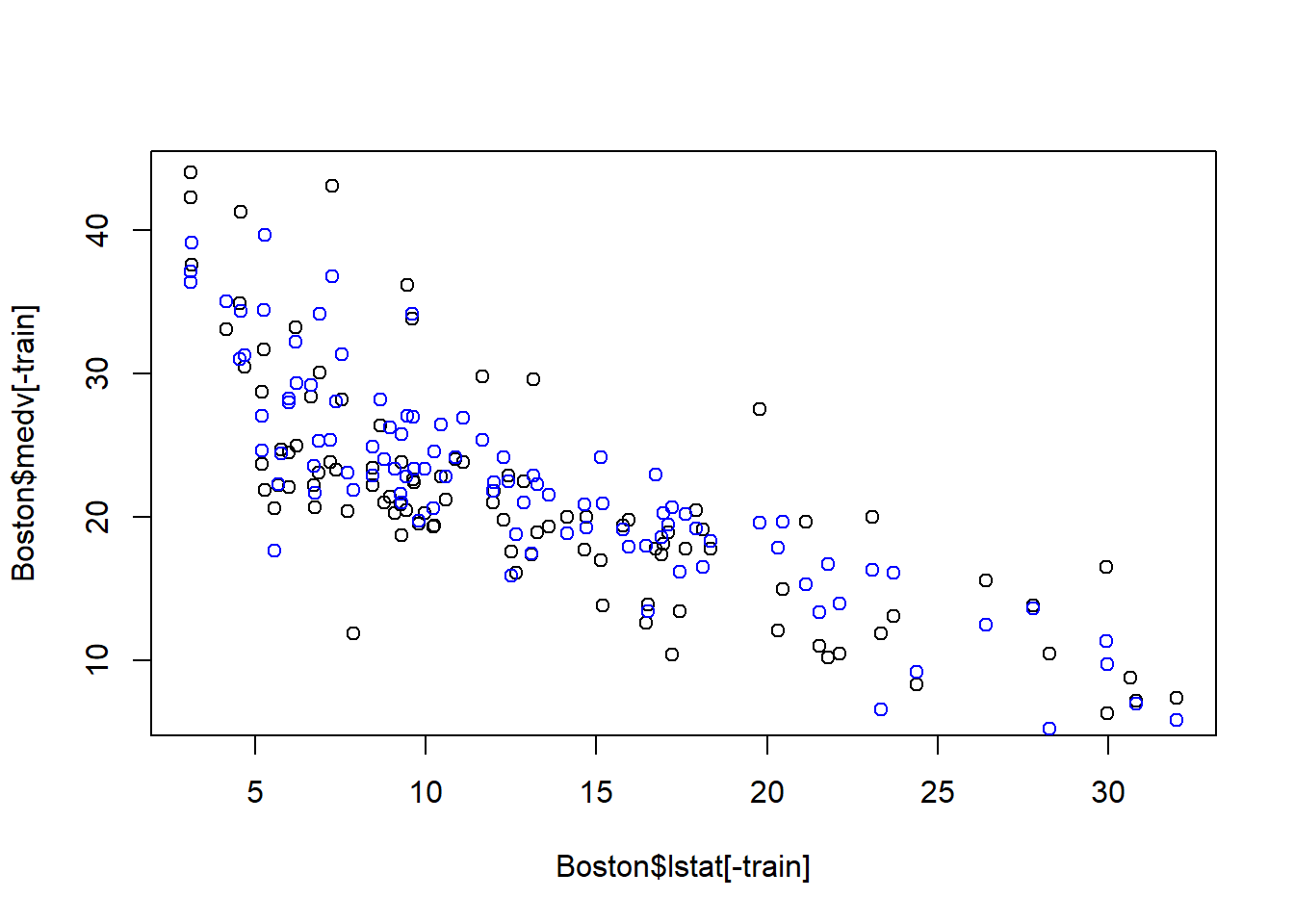
## [1] 3.237467## [1] 0.179954123.3 Exercise
# pre-process the data to include log-transformation, polynoimal terms
formula=as.formula(medv~.-lstat+log(lstat))

# find best subset based on training data
fwd_fit=regsubsets(formula, data=Boston[train,], nvmax=18, method="forward")
fwd_fit_sum=summary(fwd_fit)
fwd_fit_sum
## Subset selection object
## Call: regsubsets.formula(formula, data = Boston[train, ], nvmax = 18,
## method = "forward")
## 16 Variables (and intercept)
## Forced in Forced out
## crim FALSE FALSE
## zn FALSE FALSE
## indus FALSE FALSE
## chas1 FALSE FALSE
## nox FALSE FALSE
## rm FALSE FALSE
## age FALSE FALSE
## dis FALSE FALSE
## rad FALSE FALSE
## tax FALSE FALSE
## ptratio FALSE FALSE
## black FALSE FALSE
## locationnorth FALSE FALSE
## locationsouth FALSE FALSE
## locationwest FALSE FALSE
## log(lstat) FALSE FALSE
## 1 subsets of each size up to 16
## Selection Algorithm: forward
## crim zn indus chas1 nox rm age dis rad tax ptratio black
## 1 ( 1 ) " " " " " " " " " " " " " " " " " " " " " " " "
## 2 ( 1 ) " " " " " " " " " " "*" " " " " " " " " " " " "
## 3 ( 1 ) " " " " " " " " " " "*" " " "*" " " " " " " " "
## 4 ( 1 ) " " " " " " " " " " "*" " " "*" " " " " "*" " "
## 5 ( 1 ) " " " " " " " " " " "*" " " "*" " " " " "*" "*"
## 6 ( 1 ) " " " " " " "*" " " "*" " " "*" " " " " "*" "*"
## 7 ( 1 ) " " " " " " "*" "*" "*" " " "*" " " " " "*" "*"
## 8 ( 1 ) " " " " " " "*" "*" "*" " " "*" " " " " "*" "*"
## 9 ( 1 ) " " " " " " "*" "*" "*" " " "*" "*" " " "*" "*"
## 10 ( 1 ) "*" " " " " "*" "*" "*" " " "*" "*" " " "*" "*"
## 11 ( 1 ) "*" " " " " "*" "*" "*" "*" "*" "*" " " "*" "*"
## 12 ( 1 ) "*" "*" " " "*" "*" "*" "*" "*" "*" " " "*" "*"
## 13 ( 1 ) "*" "*" "*" "*" "*" "*" "*" "*" "*" " " "*" "*"
## 14 ( 1 ) "*" "*" "*" "*" "*" "*" "*" "*" "*" " " "*" "*"
## 15 ( 1 ) "*" "*" "*" "*" "*" "*" "*" "*" "*" " " "*" "*"
## 16 ( 1 ) "*" "*" "*" "*" "*" "*" "*" "*" "*" "*" "*" "*"
## locationnorth locationsouth locationwest log(lstat)
## 1 ( 1 ) " " " " " " "*"
## 2 ( 1 ) " " " " " " "*"
## 3 ( 1 ) " " " " " " "*"
## 4 ( 1 ) " " " " " " "*"
## 5 ( 1 ) " " " " " " "*"
## 6 ( 1 ) " " " " " " "*"
## 7 ( 1 ) " " " " " " "*"
## 8 ( 1 ) "*" " " " " "*"
## 9 ( 1 ) "*" " " " " "*"
## 10 ( 1 ) "*" " " " " "*"
## 11 ( 1 ) "*" " " " " "*"
## 12 ( 1 ) "*" " " " " "*"
## 13 ( 1 ) "*" " " " " "*"
## 14 ( 1 ) "*" "*" " " "*"
## 15 ( 1 ) "*" "*" "*" "*"
## 16 ( 1 ) "*" "*" "*" "*"# Construct test set in the same format of training set:
test_set=model.matrix(formula, data=Boston[-train,])
head(test_set)## (Intercept) crim zn indus chas1 nox rm age dis rad tax ptratio
## 1 1 0.02985 0.0 2.18 0 0.458 6.430 58.7 6.0622 3 222 18.7
## 2 1 0.08829 12.5 7.87 0 0.524 6.012 66.6 5.5605 5 311 15.2
## 3 1 0.21124 12.5 7.87 0 0.524 5.631 100.0 6.0821 5 311 15.2
## 4 1 0.17004 12.5 7.87 0 0.524 6.004 85.9 6.5921 5 311 15.2
## 5 1 0.22489 12.5 7.87 0 0.524 6.377 94.3 6.3467 5 311 15.2
## 6 1 0.11747 12.5 7.87 0 0.524 6.009 82.9 6.2267 5 311 15.2
## black locationnorth locationsouth locationwest log(lstat)
## 1 394.12 0 1 0 1.650580
## 2 395.60 0 0 1 2.520113
## 3 386.63 1 0 0 3.398861
## 4 386.71 1 0 0 2.839078
## 5 392.52 1 0 0 3.017983
## 6 396.90 1 0 0 2.585506Note: model.matrix() is a function to create a matrix which has the same columns as the regression dataset based on a formula.
Compute the out-of-sample prediction error based on test set:
#Initialize the vector for saving the mse (mean square error) err over the test set:
test_set_mse=rep(NA,16)

for(i in 1:16){

  coefi=coef(fwd_fit,id=i)
  pred=test_set[,names(coefi)]%*%coefi
  test_set_mse[i]=mean((Boston$medv[-train]-pred)^2)

}
Calculate rMSE and choose the best model to minimize rMSE:
test_set_rmse=sqrt(test_set_mse)

plot(test_set_rmse,ylab="Root MSE", type="b")

opt_id=which.min(test_set_rmse)

points(opt_id,test_set_rmse[opt_id],pch=20,col="red")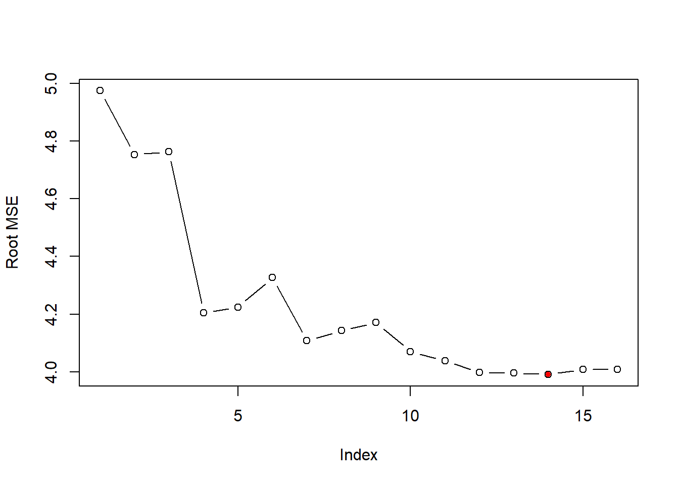
Plot the optimal out-of-sample prediction:
# obtain the model parameter for the best model
coefi=coef(fwd_fit,id=opt_id)

opt_pred=test_set[,names(coefi)]%*%coefi

plot(Boston$lstat[-train], Boston$medv[-train])
points(Boston$lstat[-train], opt_pred,col="blue")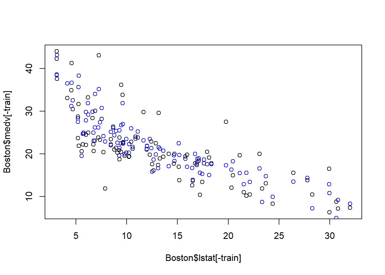
## [1] 3.075017## [1] 0.1634978