Chapter 12 Data Cleaning I

Guess what, data scientists spend 80% of their time cleaning data! When you are in a real job, the data you get to work with can be very messy. However, we do not typically teach how to clean data in class but provide students with clean data that is ready for analysis. I am compelled to teach you how to clean data, because, again, 80% of the time, we will be cleaning data. You will find the skills of cleaning data will be of great help later in your work. Thus, data cleaning, although may be tedious, will pay off in the near future.

This chapter provides a very basic introduction to cleaning data in R using the data.table, lubridate, and stringr packages. After taking the course you’ll be able to go from raw data to awesome insights as quickly and painlessly as possible!

There are two main characteristics of a clean data: 1). each row represents an observation and each column represents a variable/attribute associated with the observation. 2). The columns are in the right variable mode (e.g., numbers are numeric, date are date not character, categorical variables are factors).

Although this sounds really intuitive and simple, most raw datasets are not like that, potentially due to the way the data are collected.

There are three basic steps to clean a messy data:

exploring raw data to diagnose the places to be cleaned
tidying data to make rows as observations, columns as variables.
preparing data for analysis (converting columns into the right variable type) We will go over each of these steps in this chapter.

Run the code to install the packages (only need to run once):

install.packages("lubridate")   # dealing date variable
install.packages("stringr")     # dealing strings/character
install.packages("tidyr")       # tidying data
install.packages("data.table")

Run the code to load the packages into R:

library(lubridate)
library(stringr)
library(tidyr)

## Warning: package 'tidyr' was built under R version 4.0.5

## 
## Attaching package: 'tidyr'

## The following object is masked from 'package:magrittr':
## 
##     extract

library(data.table)

For the purpose of illustration, we will use a messy, real-world dataset containing an entire year’s worth of weather data from Boston (i.e., “weather_boston.csv”). Among other things, you’ll be presented with variables that contain column names, column names that should be values, numbers coded as character strings, and values that are missing, extreme, and downright erroneous!

First thing first, let’s read the weather_boston.csv data into R.

# use fread() to read csv into R as data.table
weather_boston<-fread("data/weather_boston.csv")

12.1 Exploring the raw data

It is critical to explore the raw data, understand its structure and diagnose why the data is messy. We can explore the raw data through the following means.

understand the structure of the data
look at the data
visualize the data

12.1.1 Understand the structure of the data

class(weather_boston) # view its class

## [1] "data.table" "data.frame"

dim(weather_boston)    # view its dimensions

## [1] 286  34

names(weather_boston)  # check the column names (variable names)

##  [1] "year"    "month"   "measure" "X1"      "X2"      "X3"      "X4"     
##  [8] "X5"      "X6"      "X7"      "X8"      "X9"      "X10"     "X11"    
## [15] "X12"     "X13"     "X14"     "X15"     "X16"     "X17"     "X18"    
## [22] "X19"     "X20"     "X21"     "X22"     "X23"     "X24"     "X25"    
## [29] "X26"     "X27"     "X28"     "X29"     "X30"     "X31"

str(weather_boston)    # examine the structure of the data

## Classes 'data.table' and 'data.frame':   286 obs. of  34 variables:
##  $ year   : int  2014 2014 2014 2014 2014 2014 2014 2014 2014 2014 ...
##  $ month  : int  12 12 12 12 12 12 12 12 12 12 ...
##  $ measure: chr  "Max.TemperatureF" "Mean.TemperatureF" "Min.TemperatureF" "Max.Dew.PointF" ...
##  $ X1     : chr  "64" "52" "39" "46" ...
##  $ X2     : chr  "42" "38" "33" "40" ...
##  $ X3     : chr  "51" "44" "37" "49" ...
##  $ X4     : chr  "43" "37" "30" "24" ...
##  $ X5     : chr  "42" "34" "26" "37" ...
##  $ X6     : chr  "45" "42" "38" "45" ...
##  $ X7     : chr  "38" "30" "21" "36" ...
##  $ X8     : chr  "29" "24" "18" "28" ...
##  $ X9     : chr  "49" "39" "29" "49" ...
##  $ X10    : chr  "48" "43" "38" "45" ...
##  $ X11    : chr  "39" "36" "32" "37" ...
##  $ X12    : chr  "39" "35" "31" "28" ...
##  $ X13    : chr  "42" "37" "32" "28" ...
##  $ X14    : chr  "45" "39" "33" "29" ...
##  $ X15    : chr  "42" "37" "32" "33" ...
##  $ X16    : chr  "44" "40" "35" "42" ...
##  $ X17    : chr  "49" "45" "41" "46" ...
##  $ X18    : chr  "44" "40" "36" "34" ...
##  $ X19    : chr  "37" "33" "29" "25" ...
##  $ X20    : chr  "36" "32" "27" "30" ...
##  $ X21    : chr  "36" "33" "30" "30" ...
##  $ X22    : chr  "44" "39" "33" "39" ...
##  $ X23    : chr  "47" "45" "42" "45" ...
##  $ X24    : chr  "46" "44" "41" "46" ...
##  $ X25    : chr  "59" "52" "44" "58" ...
##  $ X26    : chr  "50" "44" "37" "31" ...
##  $ X27    : chr  "52" "45" "38" "34" ...
##  $ X28    : chr  "52" "46" "40" "42" ...
##  $ X29    : chr  "41" "36" "30" "26" ...
##  $ X30    : chr  "30" "26" "22" "10" ...
##  $ X31    : chr  "30" "25" "20" "8" ...
##  - attr(*, ".internal.selfref")=<externalptr>

summary(weather_boston) # examine potential outliers and missing values

##       year          month          measure               X1           
##  Min.   :2014   Min.   : 1.000   Length:286         Length:286        
##  1st Qu.:2015   1st Qu.: 4.000   Class :character   Class :character  
##  Median :2015   Median : 7.000   Mode  :character   Mode  :character  
##  Mean   :2015   Mean   : 6.923                                        
##  3rd Qu.:2015   3rd Qu.:10.000                                        
##  Max.   :2015   Max.   :12.000                                        
##       X2                 X3                 X4                 X5           
##  Length:286         Length:286         Length:286         Length:286        
##  Class :character   Class :character   Class :character   Class :character  
##  Mode  :character   Mode  :character   Mode  :character   Mode  :character  
##                                                                             
##                                                                             
##                                                                             
##       X6                 X7                 X8                 X9           
##  Length:286         Length:286         Length:286         Length:286        
##  Class :character   Class :character   Class :character   Class :character  
##  Mode  :character   Mode  :character   Mode  :character   Mode  :character  
##                                                                             
##                                                                             
##                                                                             
##      X10                X11                X12                X13           
##  Length:286         Length:286         Length:286         Length:286        
##  Class :character   Class :character   Class :character   Class :character  
##  Mode  :character   Mode  :character   Mode  :character   Mode  :character  
##                                                                             
##                                                                             
##                                                                             
##      X14                X15                X16                X17           
##  Length:286         Length:286         Length:286         Length:286        
##  Class :character   Class :character   Class :character   Class :character  
##  Mode  :character   Mode  :character   Mode  :character   Mode  :character  
##                                                                             
##                                                                             
##                                                                             
##      X18                X19                X20                X21           
##  Length:286         Length:286         Length:286         Length:286        
##  Class :character   Class :character   Class :character   Class :character  
##  Mode  :character   Mode  :character   Mode  :character   Mode  :character  
##                                                                             
##                                                                             
##                                                                             
##      X22                X23                X24                X25           
##  Length:286         Length:286         Length:286         Length:286        
##  Class :character   Class :character   Class :character   Class :character  
##  Mode  :character   Mode  :character   Mode  :character   Mode  :character  
##                                                                             
##                                                                             
##                                                                             
##      X26                X27                X28                X29           
##  Length:286         Length:286         Length:286         Length:286        
##  Class :character   Class :character   Class :character   Class :character  
##  Mode  :character   Mode  :character   Mode  :character   Mode  :character  
##                                                                             
##                                                                             
##                                                                             
##      X30                X31           
##  Length:286         Length:286        
##  Class :character   Class :character  
##  Mode  :character   Mode  :character  
##                                       
##                                       
##

12.1.2 Visulize the data in Tabular form

There is no substitute to actually “see” the data. First, let’s see the data in a tabular form.

head(weather_boston)  # view the first 6 rows of the data

##    year month           measure X1 X2 X3 X4 X5 X6 X7 X8 X9 X10 X11 X12 X13 X14
## 1: 2014    12  Max.TemperatureF 64 42 51 43 42 45 38 29 49  48  39  39  42  45
## 2: 2014    12 Mean.TemperatureF 52 38 44 37 34 42 30 24 39  43  36  35  37  39
## 3: 2014    12  Min.TemperatureF 39 33 37 30 26 38 21 18 29  38  32  31  32  33
## 4: 2014    12    Max.Dew.PointF 46 40 49 24 37 45 36 28 49  45  37  28  28  29
## 5: 2014    12    MeanDew.PointF 40 27 42 21 25 40 20 16 41  39  31  27  26  27
## 6: 2014    12     Min.DewpointF 26 17 24 13 12 36 -3  3 28  37  27  25  24  25
##    X15 X16 X17 X18 X19 X20 X21 X22 X23 X24 X25 X26 X27 X28 X29 X30 X31
## 1:  42  44  49  44  37  36  36  44  47  46  59  50  52  52  41  30  30
## 2:  37  40  45  40  33  32  33  39  45  44  52  44  45  46  36  26  25
## 3:  32  35  41  36  29  27  30  33  42  41  44  37  38  40  30  22  20
## 4:  33  42  46  34  25  30  30  39  45  46  58  31  34  42  26  10   8
## 5:  29  36  41  30  22  24  27  34  42  44  43  29  31  35  20   4   5
## 6:  27  30  32  26  20  20  25  25  37  41  29  28  29  27  10  -6   1

head(weather_boston, 10)   # view the first 10 rows of the data

##     year month                  measure    X1    X2   X3    X4    X5    X6
##  1: 2014    12         Max.TemperatureF    64    42   51    43    42    45
##  2: 2014    12        Mean.TemperatureF    52    38   44    37    34    42
##  3: 2014    12         Min.TemperatureF    39    33   37    30    26    38
##  4: 2014    12           Max.Dew.PointF    46    40   49    24    37    45
##  5: 2014    12           MeanDew.PointF    40    27   42    21    25    40
##  6: 2014    12            Min.DewpointF    26    17   24    13    12    36
##  7: 2014    12             Max.Humidity    74    92  100    69    85   100
##  8: 2014    12            Mean.Humidity    63    72   79    54    66    93
##  9: 2014    12             Min.Humidity    52    51   57    39    47    85
## 10: 2014    12 Max.Sea.Level.PressureIn 30.45 30.71 30.4 30.56 30.68 30.42
##        X7    X8    X9   X10   X11   X12   X13   X14   X15   X16   X17   X18
##  1:    38    29    49    48    39    39    42    45    42    44    49    44
##  2:    30    24    39    43    36    35    37    39    37    40    45    40
##  3:    21    18    29    38    32    31    32    33    32    35    41    36
##  4:    36    28    49    45    37    28    28    29    33    42    46    34
##  5:    20    16    41    39    31    27    26    27    29    36    41    30
##  6:    -3     3    28    37    27    25    24    25    27    30    32    26
##  7:    92    92   100   100    92    85    75    82    89    96   100    89
##  8:    61    70    93    95    87    75    65    68    75    85    85    73
##  9:    29    47    86    89    82    64    55    53    60    73    70    57
## 10: 30.69 30.77 30.51 29.58 29.81 29.88 29.86 29.91 30.15 30.17 29.91 29.87
##       X19   X20   X21  X22   X23   X24   X25   X26   X27   X28   X29   X30
##  1:    37    36    36   44    47    46    59    50    52    52    41    30
##  2:    33    32    33   39    45    44    52    44    45    46    36    26
##  3:    29    27    30   33    42    41    44    37    38    40    30    22
##  4:    25    30    30   39    45    46    58    31    34    42    26    10
##  5:    22    24    27   34    42    44    43    29    31    35    20     4
##  6:    20    20    25   25    37    41    29    28    29    27    10    -6
##  7:    69    89    85   89   100   100   100    70    70    76    64    50
##  8:    63    79    77   79    91    98    75    60    60    65    51    38
##  9:    56    69    69   69    82    96    49    49    50    53    37    26
## 10: 30.15 30.31 30.37 30.4 30.31 30.13 29.96 30.16 30.22 29.99 30.22 30.36
##       X31
##  1:    30
##  2:    25
##  3:    20
##  4:     8
##  5:     5
##  6:     1
##  7:    57
##  8:    44
##  9:    31
## 10: 30.32

tail(weather_boston)     # view the last 6 rows of the data

##    year month            measure   X1 X2 X3 X4 X5 X6 X7 X8 X9 X10 X11 X12 X13
## 1: 2015    12 Mean.Wind.SpeedMPH    6                                        
## 2: 2015    12  Max.Gust.SpeedMPH   17                                        
## 3: 2015    12    PrecipitationIn 0.14                                        
## 4: 2015    12         CloudCover    7                                        
## 5: 2015    12             Events Rain                                        
## 6: 2015    12     WindDirDegrees  109                                        
##    X14 X15 X16 X17 X18 X19 X20 X21 X22 X23 X24 X25 X26 X27 X28 X29 X30 X31
## 1:                                                                        
## 2:                                                                        
## 3:                                                                        
## 4:                                                                        
## 5:                                                                        
## 6:

tail(weather_boston, 10)    # view the last 10 rows of the data

##     year month              measure   X1 X2 X3 X4 X5 X6 X7 X8 X9 X10 X11 X12
##  1: 2015    12  Max.VisibilityMiles   10                                    
##  2: 2015    12 Mean.VisibilityMiles    8                                    
##  3: 2015    12  Min.VisibilityMiles    1                                    
##  4: 2015    12    Max.Wind.SpeedMPH   15                                    
##  5: 2015    12   Mean.Wind.SpeedMPH    6                                    
##  6: 2015    12    Max.Gust.SpeedMPH   17                                    
##  7: 2015    12      PrecipitationIn 0.14                                    
##  8: 2015    12           CloudCover    7                                    
##  9: 2015    12               Events Rain                                    
## 10: 2015    12       WindDirDegrees  109                                    
##     X13 X14 X15 X16 X17 X18 X19 X20 X21 X22 X23 X24 X25 X26 X27 X28 X29 X30 X31
##  1:                                                                            
##  2:                                                                            
##  3:                                                                            
##  4:                                                                            
##  5:                                                                            
##  6:                                                                            
##  7:                                                                            
##  8:                                                                            
##  9:                                                                            
## 10:

Among other things, we see that the weather_boston dataset suffers from one of the most common symptoms of messy data: column names are values. In particular, the column names X1-X31 represent days of the month, which should really be values of a new variable called day. As a result, each row is not an individual observation, but a combined observation of 31 days. Also, variables are not orginaized by columns. The measure column indicates that the multiple measure are stacked by rows. We will tidy this data into the correct form later.

12.1.3 Visualize the raw data through charts

Histgoram is a great tool to see the range and distribution of the data. It provides a great way to identify potential outliers in your data.

hist(as.numeric(weather_boston$X1))

## Warning in hist(as.numeric(weather_boston$X1)): NAs introduced by coercion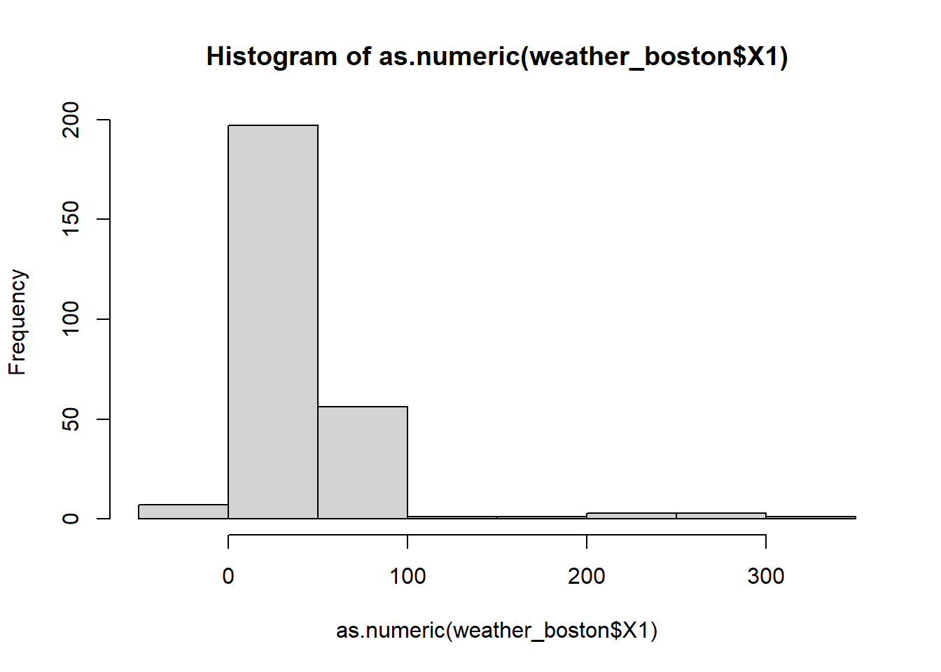

We can also look at the scatter plot between two variable to check their relationship.

plot(as.numeric(weather_boston$X1), as.numeric(weather_boston$X2))

## Warning in plot(as.numeric(weather_boston$X1), as.numeric(weather_boston$X2)):
## NAs introduced by coercion

## Warning in xy.coords(x, y, xlabel, ylabel, log): NAs introduced by coercion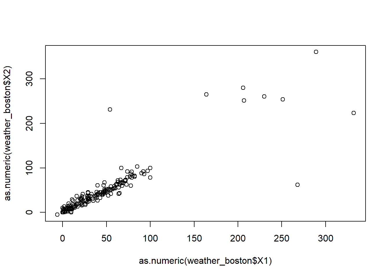

We can also look at the boxplot

boxplot(as.numeric(weather_boston$X1))

## Warning in boxplot(as.numeric(weather_boston$X1)): NAs introduced by coercion

12.2 Tidying data

What is tidy data? For any statistical analysis or visualization, the data needs to be in the right form: each row represents an observation and each column represents a variable/attribute associated with the observation. Data analyst spend huge amount of time to get data ready in this format. Nevertheless, the tidy data concept is proposed and formalized by Hadley Wickham in the Journal of Statistical Software recently. Here is the link to the paper: https://vita.had.co.nz/papers/tidy-data.pdf

Here is an example of tidy data.

country<-rep(c("United Stat", "Japan", "China"), times=3)
abbr<-rep(c("US", "JP", "CH"), times=3)
year<-rep(c(2017:2019),each=3)
GDP<-c(400,200,290,420,210,310,450,230,320)
unemployrate<-c("4%","3%","2%","4.1%","3.3%","2.5%","3.9%","3.2%","2.9%")
GDP_tidy<-data.table(country,abbr,year,GDP,unemployrate)
GDP_tidy

##        country abbr year GDP unemployrate
## 1: United Stat   US 2017 400           4%
## 2:       Japan   JP 2017 200           3%
## 3:       China   CH 2017 290           2%
## 4: United Stat   US 2018 420         4.1%
## 5:       Japan   JP 2018 210         3.3%
## 6:       China   CH 2018 310         2.5%
## 7: United Stat   US 2019 450         3.9%
## 8:       Japan   JP 2019 230         3.2%
## 9:       China   CH 2019 320         2.9%

The GDP_tidy is an example is a simple tidy data. By name, we know this data is about GDP of country. Each row represents an observation: we observe the GDP and unemployment of a particular country in a particular year. Thus, each column represents one attribute of the observation: which country is observed; in which year it is observed, and what is the observed GDP amount.

Here is an example of non-tidy data.

country<-c("United Stat/US", "Japan/JP", "China/CH")
GDP_2017<-c(400,200,290)
GDP_2018<-c(420,210,310)
GDP_2019<-c(450,230,320)
unemployrate_2017=c("4%", "3%","2%")
unemployrate_2018=c("4.1%", "3.3%","2.5%")
unemployrate_2019=c("3.9%", "3.2%","2.9%")

GDP_messy<-data.table(country,GDP_2017,GDP_2018,GDP_2019,unemployrate_2017,unemployrate_2018,unemployrate_2019)
GDP_messy

##           country GDP_2017 GDP_2018 GDP_2019 unemployrate_2017
## 1: United Stat/US      400      420      450                4%
## 2:       Japan/JP      200      210      230                3%
## 3:       China/CH      290      310      320                2%
##    unemployrate_2018 unemployrate_2019
## 1:              4.1%              3.9%
## 2:              3.3%              3.2%
## 3:              2.5%              2.9%

This is a non-tidy data because the attribute of an observation (i.e., the year when the observation is observed) is represented in the column.

Next, we will use the melt() and dcast() function in data.table package to tidy data. There are some other packages (e.g., tidyr) for this purpose. We choose to use the data.table function for consistence. Also, the data.table is very fast and memory efficient, making it well-suited to handling large data sets.

12.2.1 melt()

A common problem is a dataset where some of the column names are not names of variables, but values of a variable.

country<-c("United Stat/US", "Japan/JP", "China/CH")
abbr<-c("US", "JP", "CH")
GDP_2017<-c(400,200,290)
GDP_2018<-c(420,210,310)
GDP_2019<-c(450,230,320)

GDP_messy<-data.table(country,abbr, GDP_2017,GDP_2018,GDP_2019)
GDP_messy

##           country abbr GDP_2017 GDP_2018 GDP_2019
## 1: United Stat/US   US      400      420      450
## 2:       Japan/JP   JP      200      210      230
## 3:       China/CH   CH      290      310      320

The dataset GDP_messy from the following code as an example. The column GDP_2017, GDP_2018 and GDP_2019 represent the value of the year when it is observed.

melt() is design to collect the information in those columns name as a new variable.

GDP1<-melt(GDP_messy, id ="country", measure =c("GDP_2017","GDP_2018","GDP_2019"), variable.name = "year", value.name = "GDP")
GDP1

##           country     year GDP
## 1: United Stat/US GDP_2017 400
## 2:       Japan/JP GDP_2017 200
## 3:       China/CH GDP_2017 290
## 4: United Stat/US GDP_2018 420
## 5:       Japan/JP GDP_2018 210
## 6:       China/CH GDP_2018 310
## 7: United Stat/US GDP_2019 450
## 8:       Japan/JP GDP_2019 230
## 9:       China/CH GDP_2019 320

The code above collect the colunme name GDP_2017, GDP_2018, GDP_2019 into a new variable (and renamed as year); and put the corresponding value into the value variable (and renamed as GDP). The general format for melt() is as follow: melt( data.table, id= c("“), # id variable for origin data, will be kept in the new data measure = c(”“), # columns to be melt variable.name =”year“, # name of new variable to place original column name value.name =”GDP", # name of new variable to place original column value )

Note that: 1) the melt() function takes only data.table not data.frame as argument; 2) melt() function will return a data.table as a result; 3) the variables not included the id.vars will not be kept in the new data.table.

We can also use pattern argument:

GDP_tidy = melt(GDP_messy, id="country", measure = patterns('GDP_'),variable.name = "year", value.name = "GDP")
GDP_tidy

##           country     year GDP
## 1: United Stat/US GDP_2017 400
## 2:       Japan/JP GDP_2017 200
## 3:       China/CH GDP_2017 290
## 4: United Stat/US GDP_2018 420
## 5:       Japan/JP GDP_2018 210
## 6:       China/CH GDP_2018 310
## 7: United Stat/US GDP_2019 450
## 8:       Japan/JP GDP_2019 230
## 9:       China/CH GDP_2019 320

In the above code, instead of specifying the measure =c(“GDP_2017”,“GDP_2018”,“GDP_2019”), which share the same pattern of “GDP_”, we can use measure=patterns(‘GDP_’) to specify these columns.

To clean the data, we need extract the 4-digit year from the year column. This can be done from the following code:

GDP_tidy[,year2:=str_sub(year,5,9)]
GDP_tidy

##           country     year GDP year2
## 1: United Stat/US GDP_2017 400  2017
## 2:       Japan/JP GDP_2017 200  2017
## 3:       China/CH GDP_2017 290  2017
## 4: United Stat/US GDP_2018 420  2018
## 5:       Japan/JP GDP_2018 210  2018
## 6:       China/CH GDP_2018 310  2018
## 7: United Stat/US GDP_2019 450  2019
## 8:       Japan/JP GDP_2019 230  2019
## 9:       China/CH GDP_2019 320  2019

str_sub(year,5,9) extract the substring from the character vector year, where the position of the substring is from 5th char to the 9th char.

12.2.2 dcast()

The opposite of melt() is dcast(), which takes key-values pairs and spreads them across multiple columns. This is useful when values in a column should actually be column names (i.e. variables).

Let’s look at one example:

country<-rep(c("United Stat/US", "Japan/JP", "China/CH"), times=6)
measure<-rep(c("GDP","unemployrate"), each=3*3)
year<-rep(c(2017,2018,2019), each=3,times=2)
amount<-c("400","200","290","420","210","310","450","230","320","4%", "3%", "2%","4.1%", "3.3%", "2.5%", "3.9%", "3.2%" ,"2.9%")
GPD_messy=data.table(country,year,measure, amount)
GPD_messy

##            country year      measure amount
##  1: United Stat/US 2017          GDP    400
##  2:       Japan/JP 2017          GDP    200
##  3:       China/CH 2017          GDP    290
##  4: United Stat/US 2018          GDP    420
##  5:       Japan/JP 2018          GDP    210
##  6:       China/CH 2018          GDP    310
##  7: United Stat/US 2019          GDP    450
##  8:       Japan/JP 2019          GDP    230
##  9:       China/CH 2019          GDP    320
## 10: United Stat/US 2017 unemployrate     4%
## 11:       Japan/JP 2017 unemployrate     3%
## 12:       China/CH 2017 unemployrate     2%
## 13: United Stat/US 2018 unemployrate   4.1%
## 14:       Japan/JP 2018 unemployrate   3.3%
## 15:       China/CH 2018 unemployrate   2.5%
## 16: United Stat/US 2019 unemployrate   3.9%
## 17:       Japan/JP 2019 unemployrate   3.2%
## 18:       China/CH 2019 unemployrate   2.9%

As see, in GPD_messy, the column “measure” should be variable name: (GDP nd unemployrate are stacked in one column). We need to allocate this column into two columns. The folowing code with dcast() achieves this purpose:

GDP_tidy<-dcast(GPD_messy, country+year~measure, value.var="amount")
GDP_tidy

##           country year GDP unemployrate
## 1:       China/CH 2017 290           2%
## 2:       China/CH 2018 310         2.5%
## 3:       China/CH 2019 320         2.9%
## 4:       Japan/JP 2017 200           3%
## 5:       Japan/JP 2018 210         3.3%
## 6:       Japan/JP 2019 230         3.2%
## 7: United Stat/US 2017 400           4%
## 8: United Stat/US 2018 420         4.1%
## 9: United Stat/US 2019 450         3.9%

In the above code, country+year~measure is called formula. Here it means that each country+year pair will consists a row in the new data.table, the variables in the original “measure” column will be the new columns. value.var=“amount” indicates that the value of the new columns is populated by the value in the orignal “amount” column.

The general syntax for dcast() function is as below: dcast(data, formula, value.var).

12.3 Preparing data for analysis

Now that we have tidy the data, we need to futher clean it so that it is ready for statistical analysis or visualization. The most important task in this step is to make sure each column is in the right format (i.e., numbers are numeric, date is represented in date, categorical variables are represented in factors, characters are characters, logical are logical)

12.3.1 Type conversions

It is often necessary to change, or coerce, the way that variables in a dataset are stored. This could be because of the way they were read into R (with read.csv(), for example) or perhaps the function you are using to analyze the data requires variables to be coded a certain way.

The common type conversions in R include:

as.character(2016)

## [1] "2016"

as.numeric(TRUE)

## [1] 1

as.factor(c("level A", "level B", "leval A", "leval A"))

## [1] level A level B leval A leval A
## Levels: leval A level A level B

as.logical(0)

## [1] FALSE

Only certain coercions are allowed, but the rules for what works are generally pretty intuitive. For example, trying to convert a character string to a number gives a missing value NA:

as.numeric("some text")

## Warning: NAs introduced by coercion

## [1] NA

There are a few less intuitive results. For example, under the hood, the logical values TRUE and FALSE are coded as 1 and 0, respectively. Therefore, as.logical(1) returns TRUE and as.numeric(TRUE) returns 1.

as.logical(1)

## [1] TRUE

as.numeric(TRUE)

## [1] 1

12.3.2 Working with dates

Dates can be a challenge to work with in any programming language, but thanks to the lubridate package, working with dates in R isn’t so bad. Since this module is about cleaning data, we only cover the most basic functions from lubridate to help us standardize the format of dates and times in our data. But this will cover most of the situations you face in real world.

These functions combine the letters y, m, d, h, m, s, which stand for year, month, day, hour, minute, and second, respectively. The order of the letters in the function should match the order of the date/time you are attempting to read in, although not all combinations are valid. Notice that the functions are “smart” in that they are capable of parsing multiple formats.

# Experiment with basic lubridate functions
ymd("2015-08-25")

## [1] "2015-08-25"

class(ymd("2015-08-25"))

## [1] "Date"

ymd("2015 August 25")

## [1] "2015-08-25"

mdy("August 25, 2015")

## [1] "2015-08-25"

hms("13:33:09")

## [1] "13H 33M 9S"

ymd_hms("2015/08/25 13.33.09")

## [1] "2015-08-25 13:33:09 UTC"

As see, the these functions from lubridate package is quite smart to understand the general date in various form and return the standardized date.

12.3.3 String (character) manipulation

Here we introduce you to string manipulation in R. In many situation we have to deal with textual data, e.g., customer review, address, tweets, ….

We will use the stringr package for string manipulation, which is written Hadley Wickham. Base R contains many functions to work with strings but we’ll avoid them because they can be inconsistent, which makes them hard to remember. Instead we’ll use functions from stringr. These have more intuitive names, and all start with str_.

Examine the length of a string:

str_length(c("a", "data science", NA))

## [1]  1 12 NA

Combine two or more strings (we have used paste() in base R for this):

str_c("Leon", "Xu", sep=" ")

## [1] "Leon Xu"

str_c(2019, "Mar", 24, sep="-")

## [1] "2019-Mar-24"

str_c("https://www.zillow.com/", c("page1","page2","page3"), sep="")

## [1] "https://www.zillow.com/page1" "https://www.zillow.com/page2"
## [3] "https://www.zillow.com/page3"

subsetting strings: you can extract parts of a string use str_sub(). Subsetting a string is the most used operations to deal with strings. E.g., to extract zip from address. It takes a general form like this: str_sub(string, start, end)

address="7313 Sherman Street, Licoln, NE 68506"
len=str_length(address)

str_sub(address,  len-4, len)

## [1] "68506"

str_replace() and str_replace_all() allow you to replace matches with new strings. The general syntax is: str_replace(string, pattern, replacement)

x<-c("apple?","pear4","banana")

str_replace(x,"a","A")   # replace the first match

## [1] "Apple?" "peAr4"  "bAnana"

str_replace_all(x,"a","A")  # replace all match

## [1] "Apple?" "peAr4"  "bAnAnA"

Trim all leading and trailing whitespace

str_trim(c("   Filip ", "Nick  ", " Jonathan"))

## [1] "Filip"    "Nick"     "Jonathan"

Pad these strings with leading zeros

str_pad(c("23485W", "8823453Q", "994Z"), width=7, side='left', pad="0")

## [1] "023485W"  "8823453Q" "000994Z"

tolower() turn all letter in string into lower case.

tolower("University of Nebraska")

## [1] "university of nebraska"

toupper() turn all letter in string into upper case.

toupper("University of Nebraska")

## [1] "UNIVERSITY OF NEBRASKA"

12.4 Missing and special values in R

Missing values in R should be represented by NA.

If missing values are properly coded as NA, the is.na() function will help you find them.

Unfortunately you will not always be so lucky. Before you can deal with missing values, you have to find them in the data. Otherwise, if your dataset is too big to just look at the whole thing, you may need to try searching for some of the usual suspects like "“,”#N/A", etc to identify the missing value.

Let’s examine the example to see the missing values.

x<-data.table(x1=c(2,5,NA,9), x2=c(NA, 23,9,NA))
x

##    x1 x2
## 1:  2 NA
## 2:  5 23
## 3: NA  9
## 4:  9 NA

is.na() return for each element in the data.table, it returns TRUE/FALSE to indicate whether the data is missing.

is.na(x)

##         x1    x2
## [1,] FALSE  TRUE
## [2,] FALSE FALSE
## [3,]  TRUE FALSE
## [4,] FALSE  TRUE

# since TRUE is stored as 1 and FALSE is stored as 0, we can use sum() to count to total number of missing value
sum(is.na(x))

## [1] 3

# use which() returns the index of missing elements in each column
which(is.na(x$x1))

## [1] 3

which(is.na(x$x2))

## [1] 1 4

# Use complete.cases() to see which rows have no missing values
complete.cases(x)

## [1] FALSE  TRUE FALSE FALSE

For each row in x, complete.cases(x) returns TRUE/FALSE if the corresponding row has’t/has missing value.

# Use na.omit() to remove all rows with any missing values
na.omit(x)

##    x1 x2
## 1:  5 23

na.omit() remove all rows that contain missing value. The resulting data will have no missing value.

12.5 Outliers, obvious error and missing value

When dealing with strange values in your data, you often must decide whether they are just extreme or actually error. Extreme values show up all over the place, but you, the data analyst, must figure out when they are plausible and when they are not.

One quick way to see the outlier is to visulize your data. The summary() and hist() and boxplot() are useful for this purpose.

# Look at a summary() of a variable
summary(as.numeric(weather_boston$X1))

## Warning in summary(as.numeric(weather_boston$X1)): NAs introduced by coercion

##    Min. 1st Qu.  Median    Mean 3rd Qu.    Max.    NA's 
##   -6.00   10.00   29.99   38.70   50.00  332.00      17

# View a histogram of a variable
hist(as.numeric(weather_boston$X1), breaks=30)

## Warning in hist(as.numeric(weather_boston$X1), breaks = 30): NAs introduced by
## coercion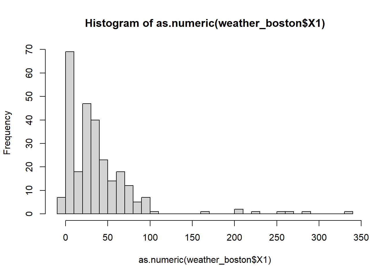

Another useful way of looking at strange values is with boxplots. Simply put, boxplots draw a box around the middle 50% of values for a given variable, with a bolded horizontal line drawn at the median. Values that fall far from the bulk of the data points (i.e. outliers) are denoted by open circles.

# view a boxplot
boxplot(as.numeric(weather_boston$X1))

## Warning in boxplot(as.numeric(weather_boston$X1)): NAs introduced by coercion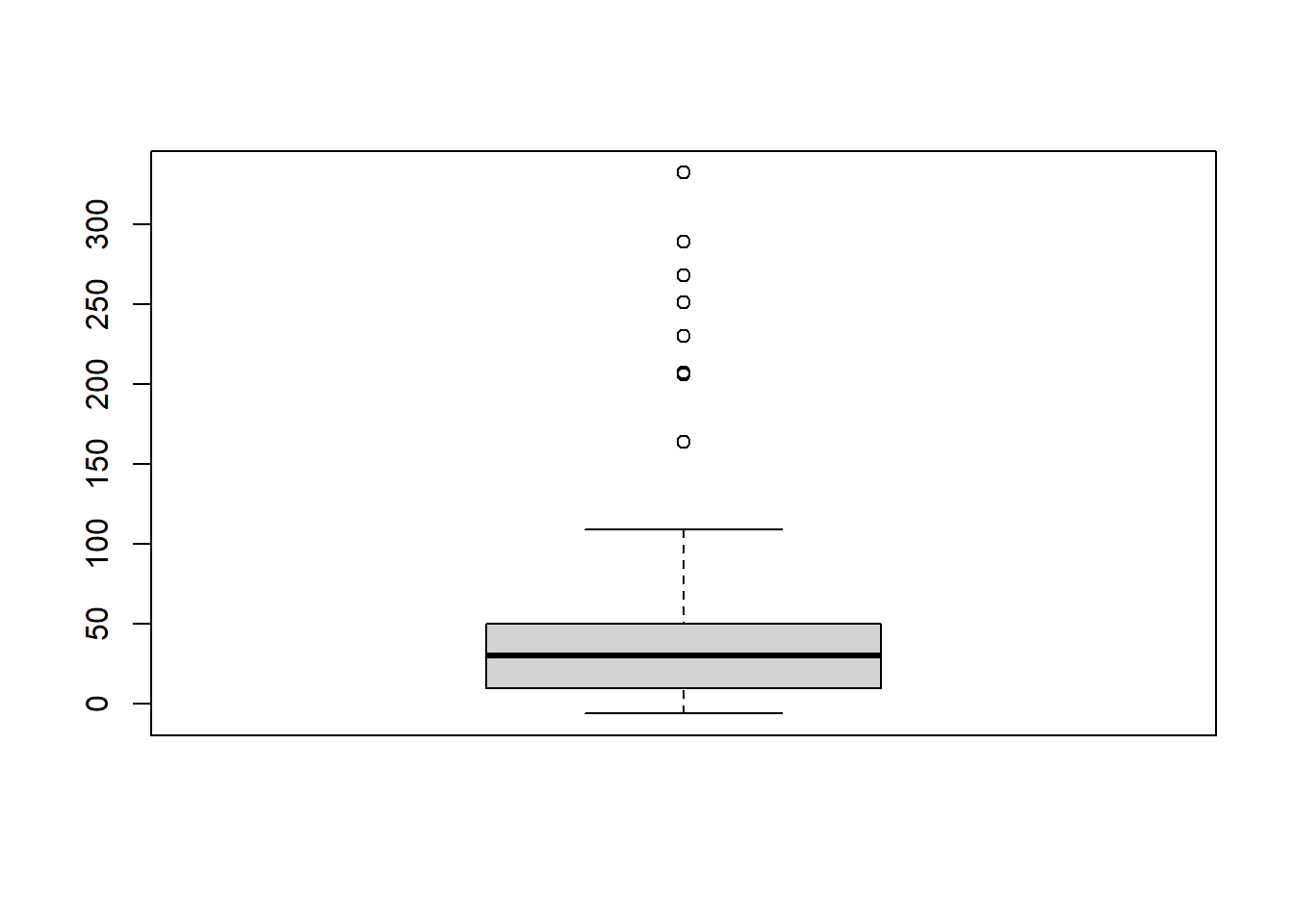

12.6 Summary

80% of the data scientist’s time is to clean data.
Three steps to clean data: 1) exploring raw data to for diagnosis; 2) tidy the data using melt() and dcast() 3) convert columns into the right variable type.
A tidy data means each row represents an observation, and each column represents a variable (attribute) about an observation. When columns names contains variable information, we should use melt(); when multiple variables are stacked into rows, we should use dcast().
Convert each column into the correct variable types using as.character(), as.numeric(), as.factor(), as.logical().
Use lubridate and stringr package to work with date and string variables.