Chapter 19 Log Tranformation and Polynomial Terms
In the previous chapter, we estimated a linear line to approximate the relationship between medv and lstat. However, the approximation is not perfect because the scatter plot seems to suggests a non-linear relationship betwee medv and lstat.
Boston=fread("data/Boston.csv")
plot(Boston$lstat,Boston$medv,
     xlab ="lstat: percent of low income population in the neighborhood",
     ylab = "medv: house price")
fit1=lm(medv~lstat, data=Boston)
points(Boston$lstat, fitted(fit1), col="blue")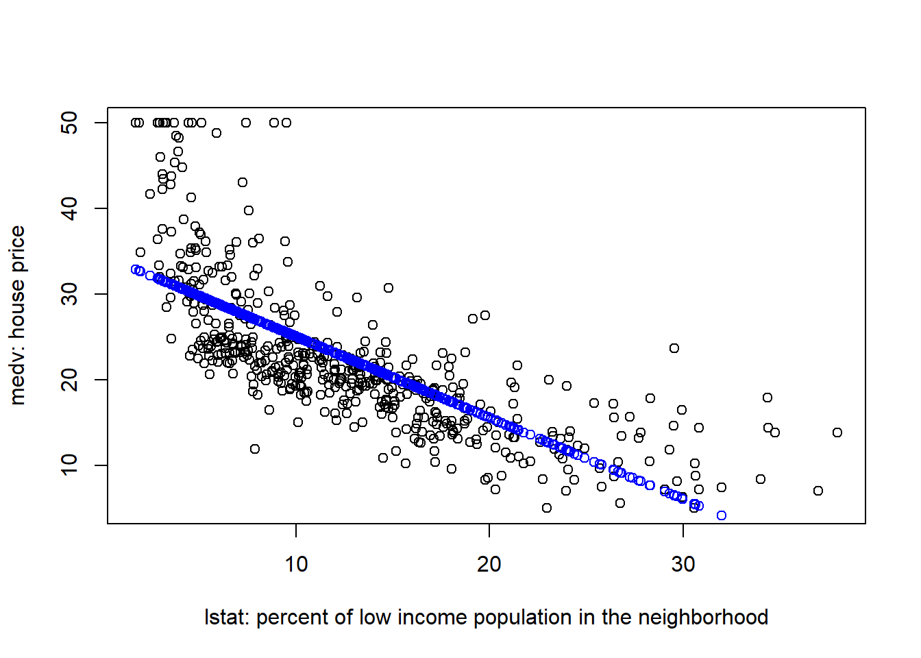
The above plot suggests that our linear model underestimated medv when lstat is either very small or very large.
There are two possible solutions to mitigate this issue:
- log-transformation
- quadratic and polynomial terms
19.1 Log-transformation
Log-transformation can be used when the dependent/independent variable is right skewed, meaning the variable does not cluster around the center (i.e., the bell shape), but has more mass on the right of the spectrum. A good way to check whether an variable is skewed is through histogram:
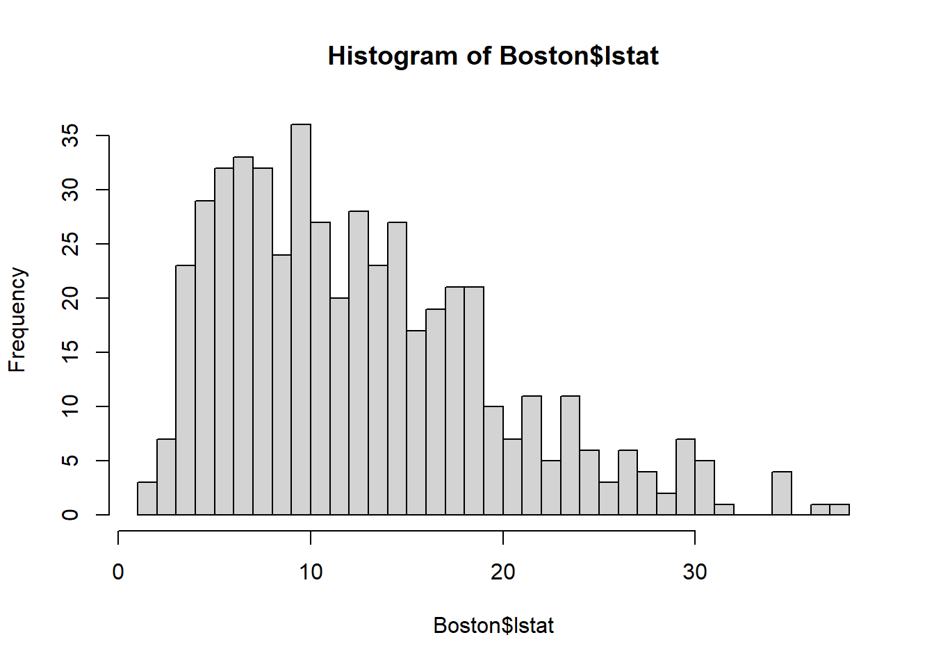
The histogram shows that lstat is right skewed since most of the mass is leaning towards right).
Now, let’s try log-transform the variable lstat and examine its histogram:
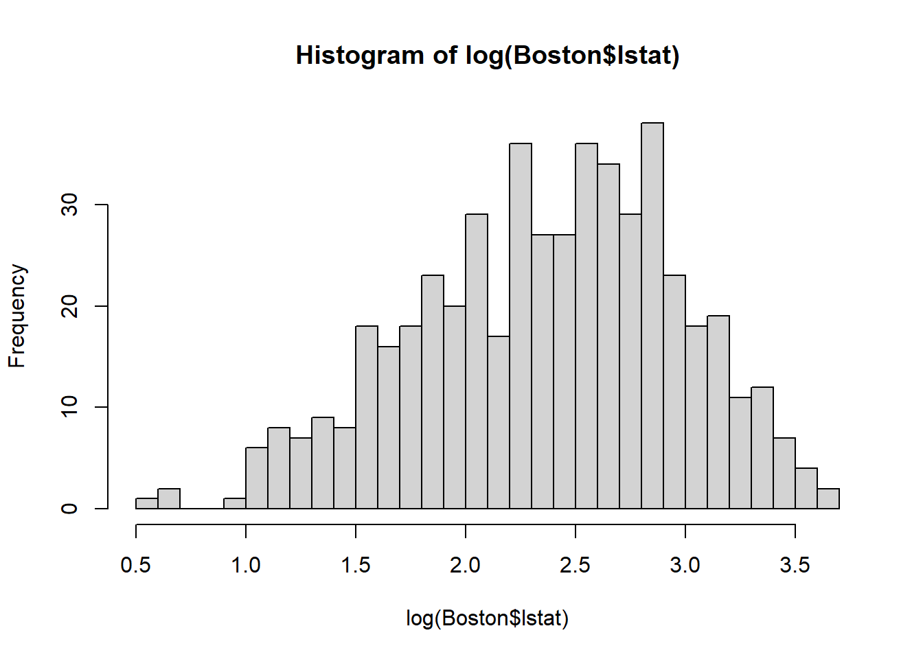
Also notice that, as a result of log-transformation, the variation in the variable is reduced (the range of lstat is 0-40; but log(lstat) is 0.5-4). Thus, the log-transformation is also widely used for reducing the variation in the data.
When the data is left-skewed, we need to use Box-cox transformation (which we will not discuss here).
Here is what the regression looks like when we log-transform the lstat variable.
##
## Call:
## lm(formula = medv ~ log(lstat), data = Boston)
##
## Residuals:
##      Min       1Q   Median       3Q      Max
## -14.4599  -3.5006  -0.6686   2.1688  26.0129
##
## Coefficients:
##             Estimate Std. Error t value Pr(>|t|)
## (Intercept)  52.1248     0.9652   54.00   <2e-16 ***
## log(lstat)  -12.4810     0.3946  -31.63   <2e-16 ***
## ---
## Signif. codes:  0 '***' 0.001 '**' 0.01 '*' 0.05 '.' 0.1 ' ' 1
##
## Residual standard error: 5.329 on 504 degrees of freedom
## Multiple R-squared:  0.6649, Adjusted R-squared:  0.6643
## F-statistic:  1000 on 1 and 504 DF,  p-value: < 2.2e-16
We can use summary() to take a quick looked the regression results. As seen, the fitted line is: \[medvFit=52.12-12.48*log(lstat)\]
Let’s plot the fitted line to see the difference.
# fitted() is the function to get the fitted value
plot(Boston$lstat, Boston$medv)
points(Boston$lstat, fitted(fit1), col="blue", type = "l")
points(Boston$lstat, fitted(fit2), col="red", cex=0.5)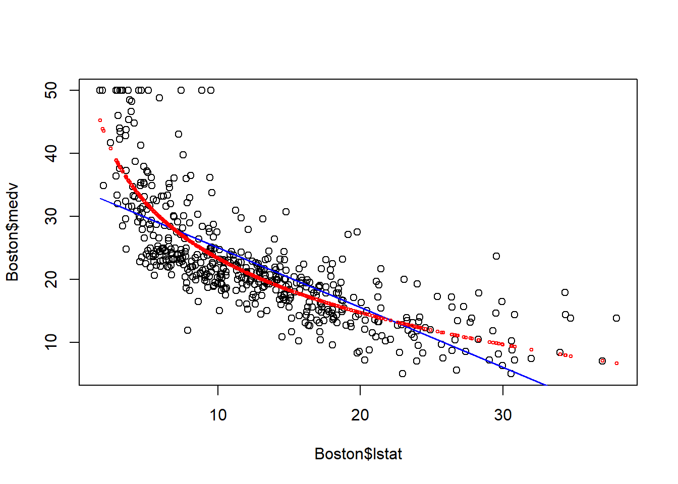 After the log transformation, the model captures the non-linear relationship between medv and lstat, and seems to provide a better fit to the data. The underestimation at both the left/right end is to some extent mitigated.
19.2 Quadratic regression
Alternatively, we can add the quadratic terms to capture the nonlinear relationship between medv and lstat.
Formally, the quadratic regression is denoted as below: \[y=\beta_0+\beta_1x+\beta_2x^2+\epsilon\] Here the quadratic term \(x^2\) is included to capture the non-linear relationship between x and y. In R, the quadratic term is represented by I(x^2).
##
## Call:
## lm(formula = medv ~ lstat + I(lstat^2), data = Boston)
##
## Residuals:
##      Min       1Q   Median       3Q      Max
## -15.2834  -3.8313  -0.5295   2.3095  25.4148
##
## Coefficients:
##              Estimate Std. Error t value Pr(>|t|)
## (Intercept) 42.862007   0.872084   49.15   <2e-16 ***
## lstat       -2.332821   0.123803  -18.84   <2e-16 ***
## I(lstat^2)   0.043547   0.003745   11.63   <2e-16 ***
## ---
## Signif. codes:  0 '***' 0.001 '**' 0.01 '*' 0.05 '.' 0.1 ' ' 1
##
## Residual standard error: 5.524 on 503 degrees of freedom
## Multiple R-squared:  0.6407, Adjusted R-squared:  0.6393
## F-statistic: 448.5 on 2 and 503 DF,  p-value: < 2.2e-16
According the estimated result, the fitted line is: \[medvFit= 42.86-2.33*lstat+0.04*lstat^2\]
Now, let’s plot the fitted line to see the difference.
plot(Boston$lstat, Boston$medv)
points(Boston$lstat, fitted(fit1), col="blue", type = "l")
points(Boston$lstat, fitted(fit2), col="red", cex=0.5)
points(Boston$lstat, fitted(fit3), col="green", cex=0.5)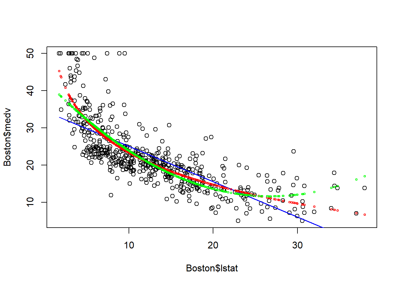
The quadartic model corrects (probably over corrects) the underestimation of medv when lstat is too small or too large. However, it may overestimate medv when lstat is large. Thus, we may want to add higher order polynomial terms to aviod that.
19.3 Polynomial regression
Polynomial is a genearlization of quadratic regression. Formally, the \(k^{th}\) order polynomial regression model is generally denoted as below: \[y=\beta_0+\beta_1x+\beta_2x^2+\beta_3x^3+...+\beta_kx^k+\epsilon\] The polynomial terms \(x^2\), …,\(x^k\) are used to capture the non-linear relationship between x and y.
This can be easily estimated in R:
##
## Call:
## lm(formula = medv ~ poly(lstat, 6), data = Boston)
##
## Residuals:
##      Min       1Q   Median       3Q      Max
## -14.7317  -3.1571  -0.6941   2.0756  26.8994
##
## Coefficients:
##                  Estimate Std. Error t value Pr(>|t|)
## (Intercept)       22.5328     0.2317  97.252  < 2e-16 ***
## poly(lstat, 6)1 -152.4595     5.2119 -29.252  < 2e-16 ***
## poly(lstat, 6)2   64.2272     5.2119  12.323  < 2e-16 ***
## poly(lstat, 6)3  -27.0511     5.2119  -5.190 3.06e-07 ***
## poly(lstat, 6)4   25.4517     5.2119   4.883 1.41e-06 ***
## poly(lstat, 6)5  -19.2524     5.2119  -3.694 0.000245 ***
## poly(lstat, 6)6    6.5088     5.2119   1.249 0.212313
## ---
## Signif. codes:  0 '***' 0.001 '**' 0.01 '*' 0.05 '.' 0.1 ' ' 1
##
## Residual standard error: 5.212 on 499 degrees of freedom
## Multiple R-squared:  0.6827, Adjusted R-squared:  0.6789
## F-statistic: 178.9 on 6 and 499 DF,  p-value: < 2.2e-16
Now, let’s plot the fitted line to see the difference.
# fitted() is the function to get the fitted value
plot(Boston$lstat, Boston$medv)
points(Boston$lstat, fitted(fit1), col="blue", type = "l")
points(Boston$lstat, fitted(fit2), col="red", cex=0.5)
points(Boston$lstat, fitted(fit3), col="green", cex=0.5)
points(Boston$lstat, fitted(fit4), col="yellow", cex=0.5)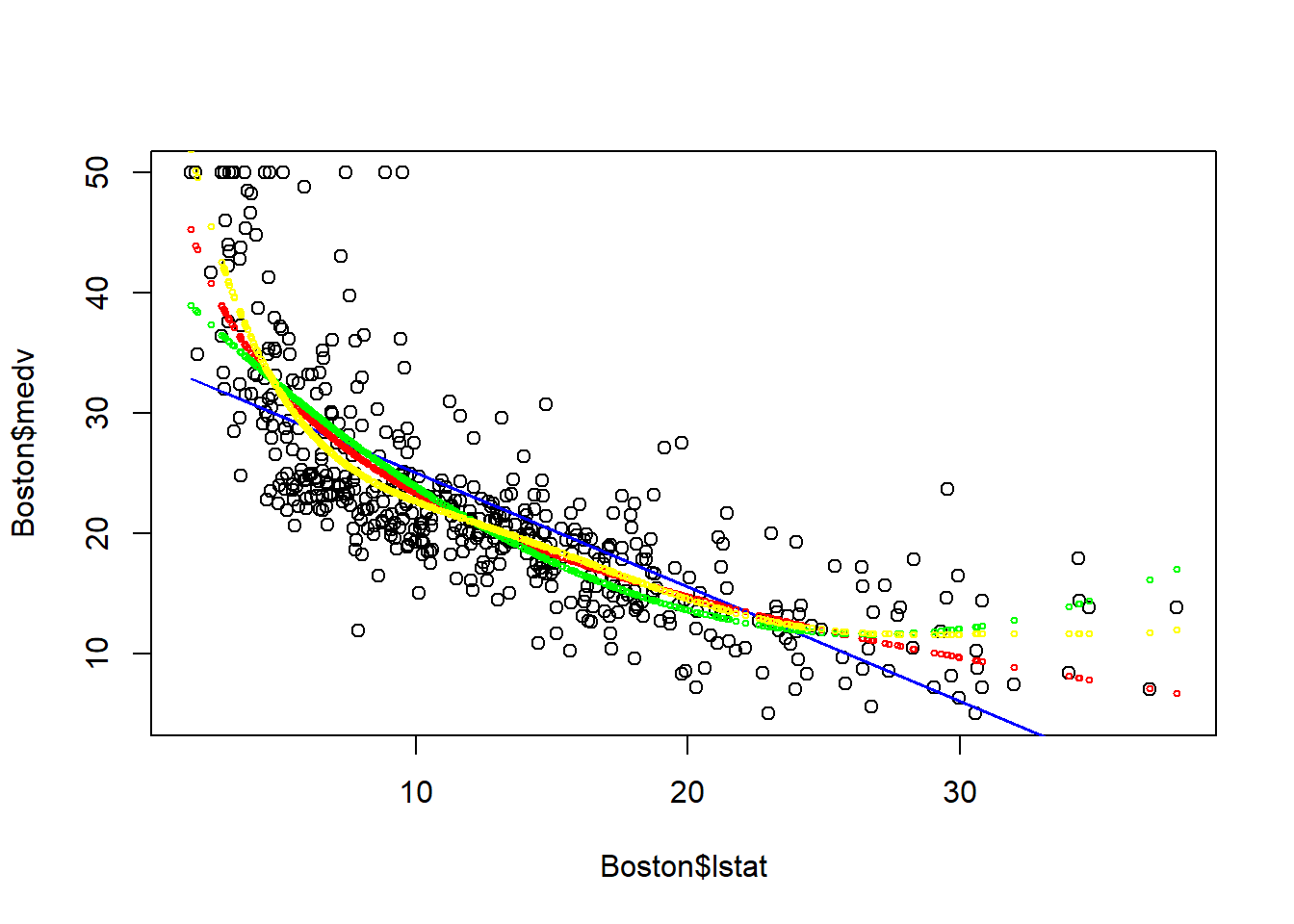 The \(6^{th}\) order polynomial regression seems to provide a good fit to the data.
You may be wondering, now we have four different model to predict medv. For a given lstat, each model predicts a differnt medv. Which model should we trust? Which model is the best model? We will come back to this question in the model selection chapter.
19.4 Summary
- log-transformation can correct the right-skewness of the variable, and reduce variation in the variable.
- We can use log-transformation and polynoimal terms to capture non-linear relationship between dependent variable and independent variables.
19.5 Exercise
Use nox (nitrogen oxides concentration (parts per 10 million)) to explain medv through a linear regression model, i.e., \[medv=\beta_0+\beta_1 nox+\epsilon\] You need to try the following models:
- Model 1: linear regression without any transformation
- Model 2: log-transformation on nox
- Model 3: add quadartic term of nox
- Model 4: \(10^{th}\) order polynomial regression
19.5.1 Solution
Let’s first examine the data visually.
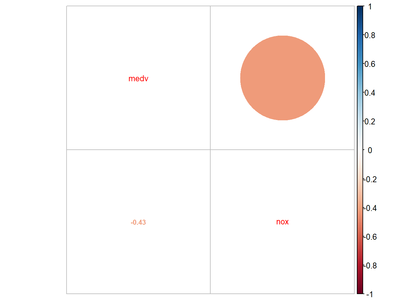
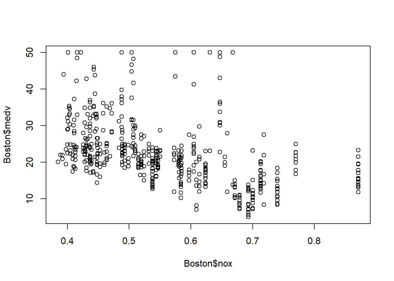
There seems to exist a negative linear relationship between nox and medv: house price in region with higher nox (more air pollution) has lower price.
Let’s quantify such linear relationship:
# estimate four different models
fit1=lm(formula=medv~nox, data=Boston)
fit2=lm(formula=medv~log(nox), data=Boston)
fit3=lm(formula=medv~nox+I(nox^2), data=Boston)
fit4=lm(formula=medv~poly(nox,10), data=Boston)

# generate the fitted value for each model
plot(Boston$nox, Boston$medv)
points(Boston$nox, fitted(fit1), col="blue", type = "l")
points(Boston$nox, fitted(fit2), col="red", cex=0.5)
points(Boston$nox, fitted(fit3), col="green", cex=0.5)
points(Boston$nox, fitted(fit4), col="yellow", cex=0.5)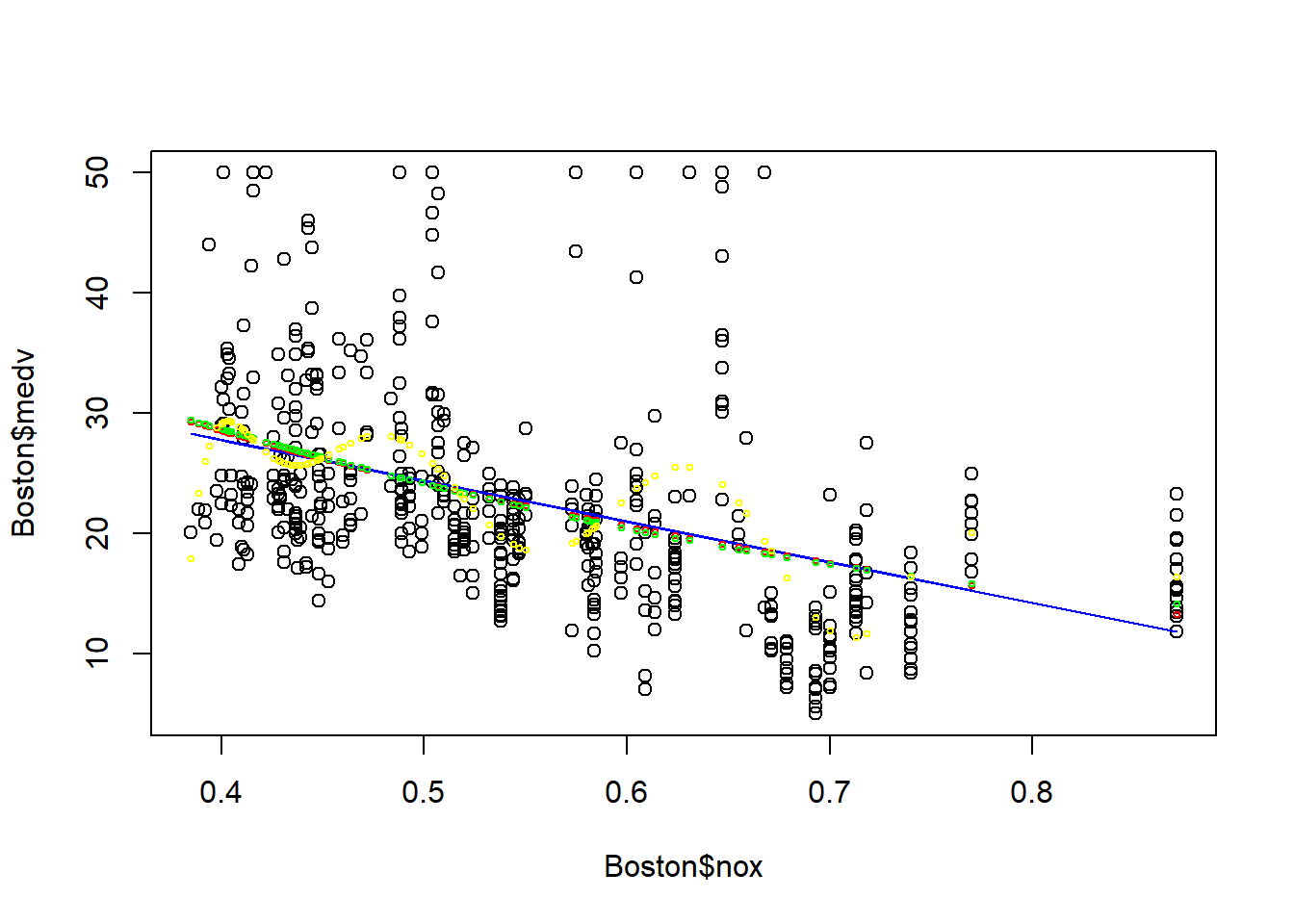
It seems model 1-3 provide similar fit, however model 4 (polynomial-10) seems to have a problem of over-fitting: the model is too specific to the training data, and cannot be generalizable for out-of-sample prediction. Thus, it is not always the best to have a complicated model. We will come back to the problem of over-fitting in the model selection chapter.